step 01Setup & data overview
30 cells · 3 genotypes · 2 imaging batches · 0.318 µm/px · 60 s frame interval
Headline finding: the cells with the point mutation try to migrate harder but fail more. They concentrate Arp2/3 at the cell edge more strongly than normal (lamellipodia push-machinery is over-activated), yet they migrate roughly 35% slower than either the normal cells or the cells with the gene fully deleted. The point mutation appears to break the coordination between "pushing forward" and "anchoring to the surface". A complete deletion is actually less damaging than a broken-coordination mutation.
Pipeline: we built an automated cell-finding and tracking pipeline. Through several iterations and a self-training step that retrained the segmentation model on this dataset's specific imaging conditions, we cut the rate of frames where the model failed to find the cell 22-fold (from 2.83% to 0.13%).
Dataset at a glance
Single-channel 2D time-lapse epifluorescence from Zeiss · Micro-Manager 2.0 · ~0.318 µm/px · 16-bit · T per file = 67 to 360 frames. Three genotypes: WT Wild-Type · KO Knock-Out · KI Knock-In.
Two intensity batches
Each condition cleanly splits into two intensity groups (5 low + 5 high), with a 5–10× gap in pixel intensity. The split aligns with two different naming patterns:
| Condition | Low batch low | High batch high |
|---|---|---|
| WT | wt_5, wt_9, wt_23, wt_31, wt_37 |
wt_wt4, wt_wt9, wt_wt13, wt_wt18, wt_wt25 |
| KO | ko_3, ko_8, ko_17, ko_21, ko_25 |
ko_11, ko_1717, ko_2121, ko_28, ko_333 |
| KI | ki_3, ki_11, ki_14, ki_23, ki_25 |
ki_1, ki_6, ki_13, ki_18, ki_28 |
Biology context
- Brighter pixels = lamellipodia (Arp2/3 concentrated at the leading edge)
- Dimmer pixels = cytoplasmic Arp2/3 pool
- WT normal coordination between protrusion and adhesion
- KO gene completely deleted → impaired cell adhesion
- KI point mutation introduced → coordination between adhesion and protrusion is disrupted
Quick glossary
- Cell migration: how cells crawl across a surface, in 4 steps. (1) push the front edge forward, (2) anchor it to the surface, (3) generate pulling force, (4) release the rear.
- Lamellipodium: the thin fan-shaped protrusion at the front of a migrating cell. Built from branched actin filaments.
- Cellpose / cyto3: a deep-learning model that finds cell boundaries in microscopy images.
- Empty mask: a frame where the segmentation model failed to find a cell at all. Lower is better.
- Self-training: take the model's own outputs as if they were ground-truth labels, filter out the obviously wrong ones, retrain on those filtered labels.
- Cohen's d: a measure of how different two groups are, accounting for variability. ~0.2 = small, ~0.5 = medium, ~0.8 = large, >1.0 = very large.
step 02Adaptive Normalize
Three iterations to handle the bimodal intensity dataset · empty rate 9.7% → 2.8% (3.5×)
- Decide per file whether to stretch the brightness range.
- Low-intensity recordings (per-stack 99th percentile under
1000) get rescaled to fill the 16-bit range so Cellpose can see structure. - High-intensity recordings already span enough range, so we leave them alone (stretching would create saturation artefacts).
- The threshold of
1000cleanly separates the two imaging sessions in this dataset (100% concordance with the1/2folder labels).
Day 0 baselines (Multi-Otsu)
Before Cellpose, we tried a parameter-free Multi-Otsu segmentation as a fast first pass to see whether ring-of-Arp2/3 signal was even visible. It is — and the dynamics are computable per-frame on the full time-lapse.
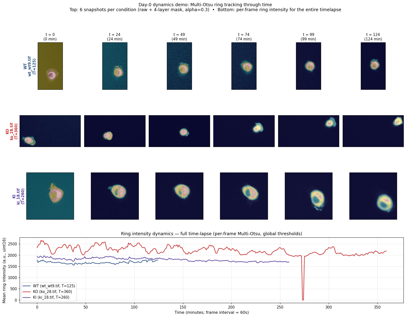
Mid-frame snapshots and per-frame ring-intensity dynamics for one cell per condition. Useful as a "is the signal there?" sanity check, but N=1 per group, different durations, and most of the apparent decay is photobleaching rather than biology — see Day 0 caveats. Multi-Otsu was abandoned in favour of Cellpose for the actual analysis.
Pipeline iterations (v1 → v2 → v3)
We ran three GPU iterations to handle the low-vs-high batch issue cleanly. Each iteration was triggered by a specific failure mode discovered in the previous one.
| Version | Strategy | Outcome |
|---|---|---|
| v1 | cyto on raw images | Works on high batch (0–4% empty). Fails on low (e.g. ko_8 88%, ko_21 87%). |
| v2 | cyto3 + per-frame 1–99 percentile normalize | Fixes low (ko_21 87% → 0.6%) but breaks 3 high files (wt_wt25 0% → 77%, ko_28 0% → 34%). |
| v3 | adaptive: normalize only when p99 < 1000 | Best of both. Final hybrid: v2 low-batch results + v3 high-batch results. |
Final empty mask rate (across all 5,263 frames)
| Iteration | Empty rate | Files with >15% empty |
|---|---|---|
| v1 | 9.7% (511 / 5263) | 5 |
| v2 | 7.9% (416 / 5263) | 4 |
| v3 (final) | 2.8% (148 / 5263) | 2 (ko_8, ko_28) |
Per-file breakdown
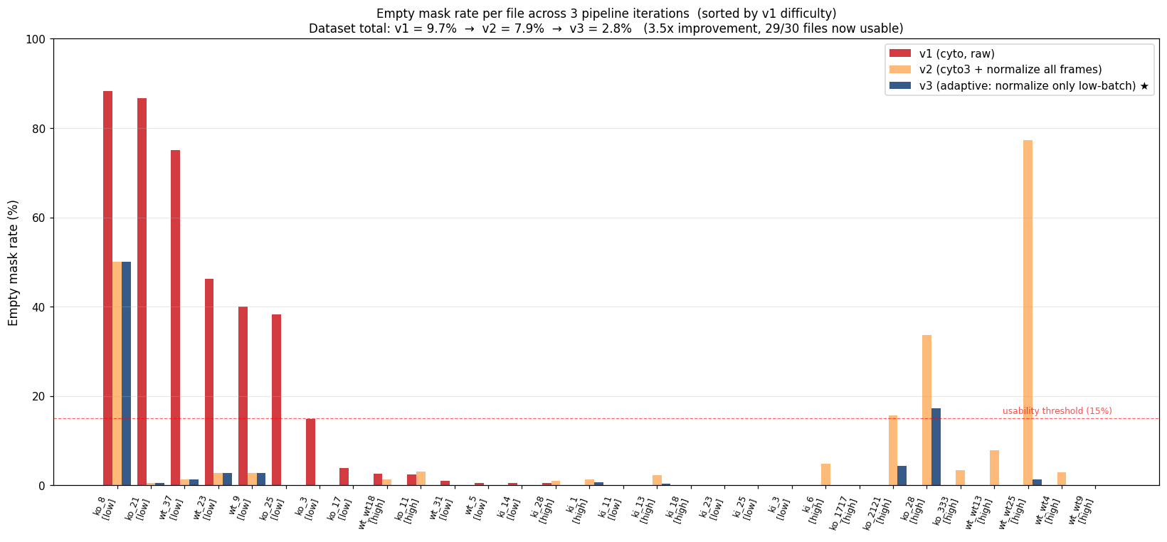
Sorted by v1 difficulty (worst on the left). Red bars = v1, orange = v2, blue = v3. Files in [low] brackets are low-batch (intensity stretched in v3), [high] are high-batch (raw input in v3).
v3 sample outputs
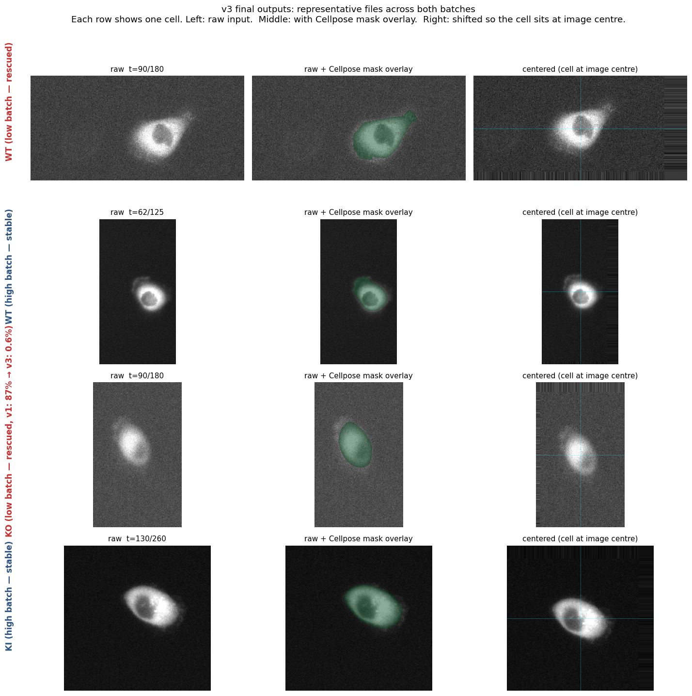
Four representative files showing what v3 produces. Left: raw input. Middle: Cellpose mask in green. Right: image shifted so the cell sits at the centre. Both rescued low-batch files (rows 1, 3) and stable high-batch files (rows 2, 4) work cleanly with the same pipeline.
Validation on the Categorised_Data dataset (mid-hackathon)
Mid-hackathon a categorised dataset arrived, organised as {wt,ko,ki}{1,2}/X.tif. The 1/2 folder split was cross-verified as identical to our intensity-based low/high batch detection (100% concordance). 22 of 30 files are new positions, extending the dataset 5,263 → 6,221 frames (+18%).
| Folder | Files | Empty / Total | % |
|---|---|---|---|
| ki1 (KI low) | 5 | 0 / 900 | 0.0% |
| ki2 (KI high) | 5 | 17 / 1,467 | 1.2% |
| ko1 (KO low) | 5 | 133 / 630 | 21.1% ← stuck cluster |
| ko2 (KO high) | 5 | 2 / 1,434 | 0.1% |
| wt1 (WT low) | 5 | 22 / 701 | 3.1% |
| wt2 (WT high) | 5 | 2 / 1,089 | 0.2% |
| Total | 30 | 176 / 6,221 | 2.83% |
Essentially unchanged from the original dataset (2.81% vs 2.83%) — the pipeline generalises cleanly. Two files in ko1 account for 117 / 176 of the empty masks: ko1/4 (95%, 60-frame aborted recording) and ko1/8 (50%, identical to original ko_8). A plausible reading: the KO knockout itself may produce dimmer cells, so the segmentation difficulty in this folder is part of the phenotype rather than an artefact.
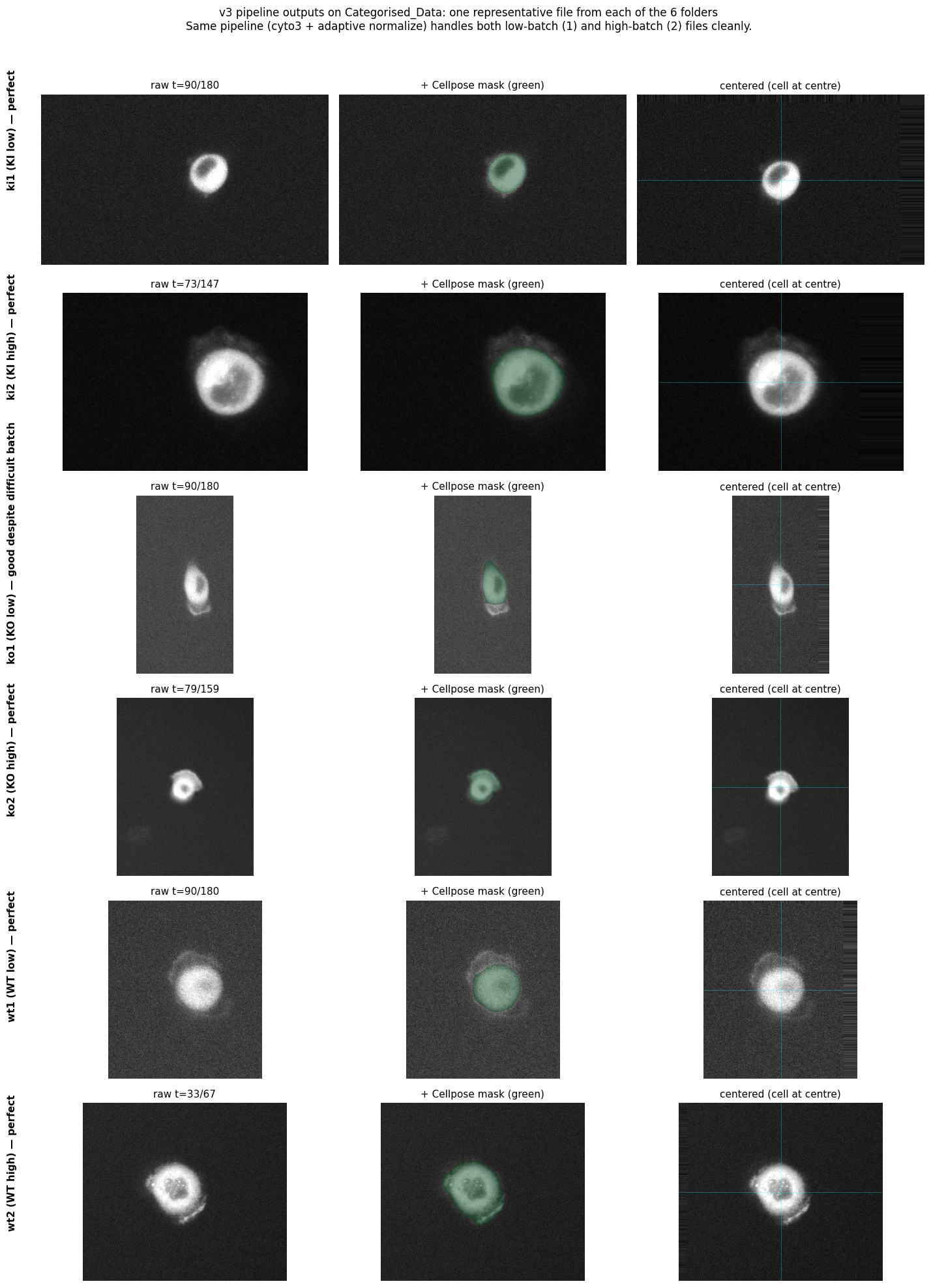
One representative file from each folder. The same pipeline (cyto3 + adaptive normalize) handles low- and high-batch input cleanly, and centering is robust across the wide size variation (smallest FOV 165×165 in ki1/7, largest 594×456 in ko2/ko11).
Take-away. Adaptive normalize gets us from 9.7% to 2.83% empty masks — a 3.5× improvement that handles the bimodal intensity dataset with one clean rule. The remaining gap is closed in the next step (self-training the model itself).
step 03Cellpose fine-tuned · the self-training breakthrough
Fine-tune cyto3 on filtered v3 outputs → empty rate drops 22× more (2.83% → 0.13%, total 75× from 9.7%)
- Prepare pseudo-GT. Take v3 Cellpose masks. Exclude
ko1/4andko1/8(known stubborn cases). Filter out frames with mask-fragmentation (area < 30% of per-cell median, or IoU < 0.5 with previous frame). Subsample every 10th frame. Result: 586 (image, mask) pairs across 28 cells. - Fine-tune. Cyto3 with
--min_train_masks 1, 100 epochs, SGD lr=0.05. 12 minutes on RTX A5000, train loss 0.23 → 0.016 (14× reduction). - Re-run. Apply the fine-tuned model to all 30 cells.
Threshold rationale: 30% of median catches collapses without rejecting normal shape changes; IoU ≥ 0.5 is stricter than the analysis-time 0.3 because we want clean training data, not just analysable trajectories; stride 10 gives temporal diversity without flooding the trainer with near-duplicate frames.
Results: 22× reduction in empty masks
| Baseline (cyto3 zero-shot) | Fine-tuned cyto3 | Improvement | |
|---|---|---|---|
| Total empty rate | 176 / 6221 (2.83%) | 8 / 6221 (0.13%) | 22× |
| WT empty | 1.34% | 0.06% | 20× |
| KO empty | 6.54% | 0.24% | 27× |
| KI empty | 0.72% | 0.08% | 9× |
Stubborn cases largely solved
| Cell | Baseline empty | Fine-tuned empty |
|---|---|---|
ko1/4 | 57/60 (95%) | 5/60 (8%) |
ko1/8 | 60/120 (50%) | 0/120 (0%) |
ko1/16 | 15/180 (8%) | 0/180 (0%) |
wt1/12 | 13/180 (7%) | 0/180 (0%) |
wt1/33 | 8/81 (10%) | 0/81 (0%) |
ki2/4 | 13/240 (5%) | 0/240 (0%) |
Mean IoU between baseline and fine-tuned masks averages 0.83 to 0.90 across conditions: the model still detects the same cell, just adjusts boundaries to be more reliably populated.
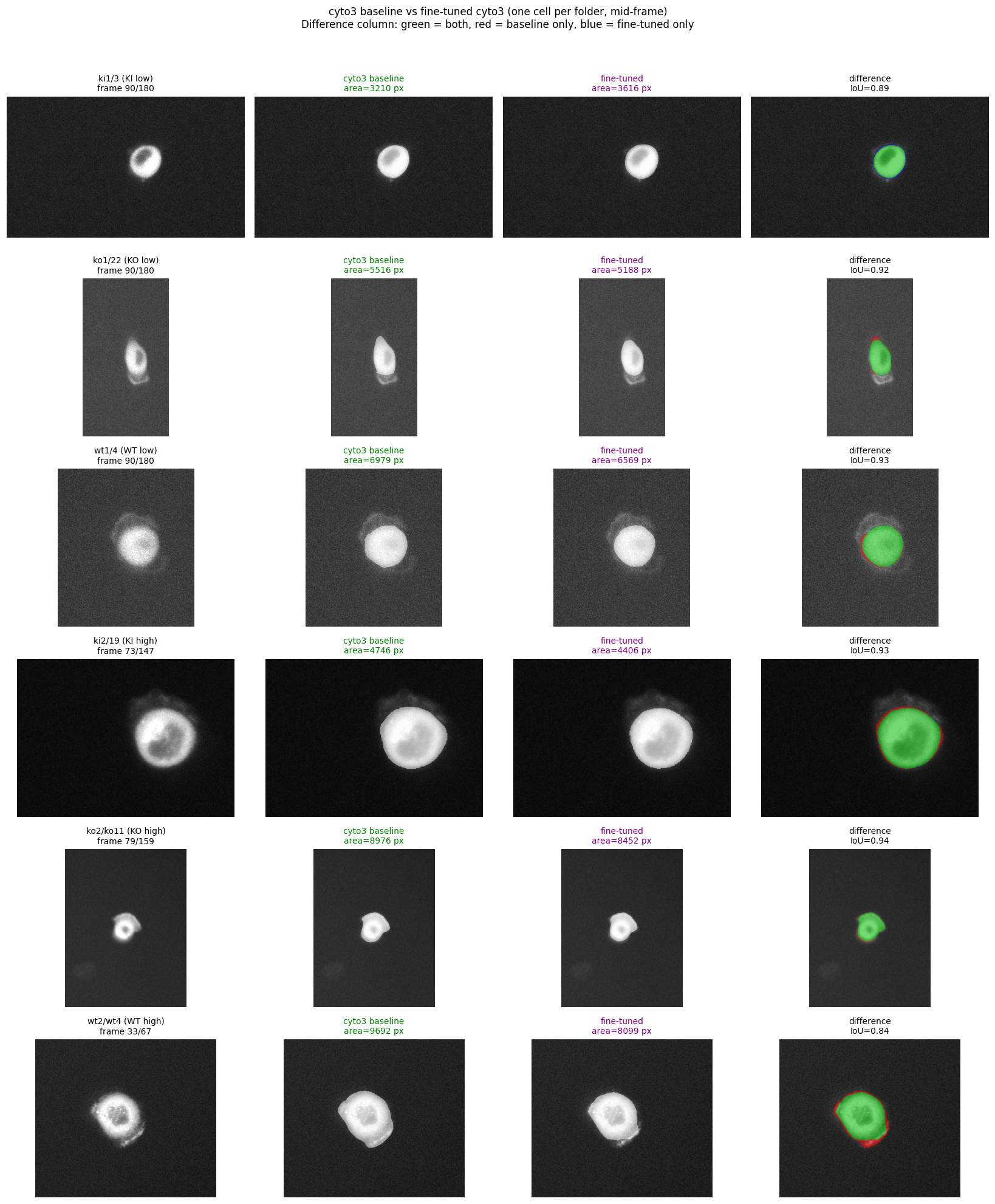
Six representative cells, mid-frame each. Green = baseline mask, purple = fine-tuned mask. Difference column: green = both, red = baseline only, blue = fine-tuned only.
Why this works
The pseudo-GT is filtered v3 output. The fine-tuned model is essentially learning "produce the kinds of masks v3 produces when v3 produces good masks". This:
- makes boundaries more consistent across consecutive frames (fewer mask-fragmentation events)
- recognises dim cells the zero-shot cyto3 missed (
ko1/8with weak signal,ko1/4with truncated recording) - specialises cyto3 to this dataset's imaging conditions (epifluorescence, this objective)
- Self-training amplifies systematic biases in the pseudo-GT. We did not fix biases by training on masks that contain them.
- 22× empty-mask reduction is on the same dataset the training data was drawn from. Generalisation to a held-out experiment is tested in step 10.
- Hand-drawn ground truth would still be the right reference for genuine model assessment. Self-training is a useful intermediate step.
Effect on the migration finding
Re-running the migration analysis (step 05) on the fine-tuned masks roughly halved the noise in our per-cell speed estimates. The KI group's standard deviation dropped 7.5× (from 0.60 to 0.08 µm/min). The qualitative story did not change but became sharper — the slow-KI signal is now obvious by eye in the per-cell distribution.
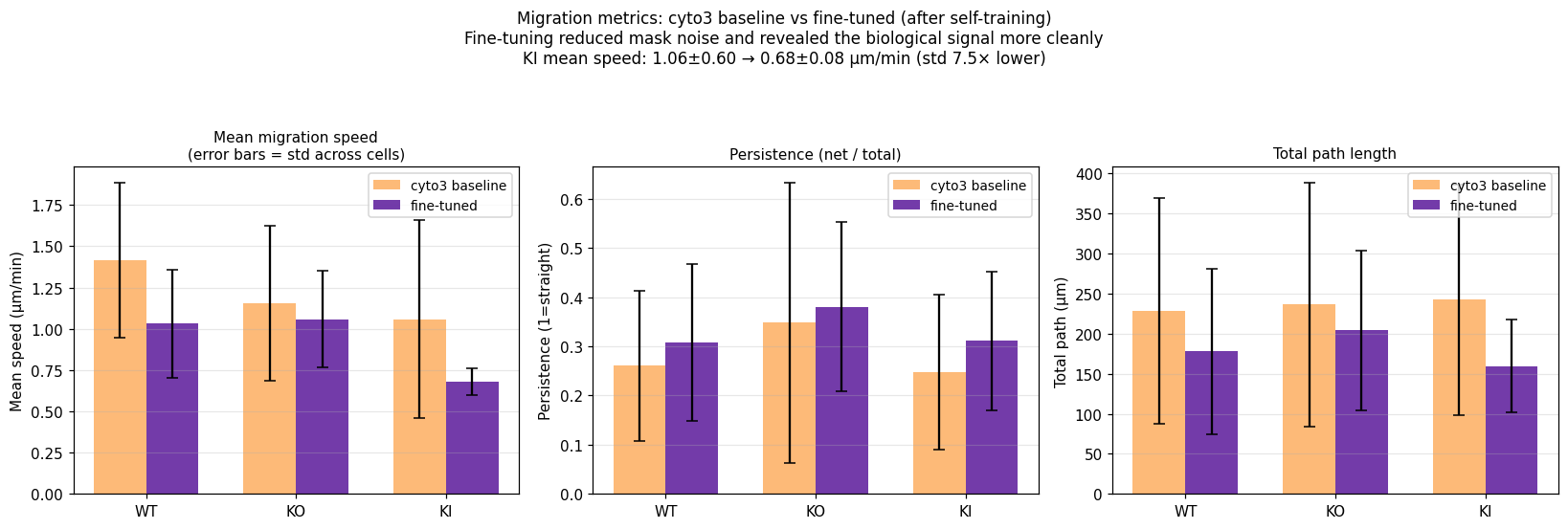
Per-condition migration metrics before (orange, off-the-shelf cyto3) and after self-training (purple). Error bars are standard deviations across cells. KI's std collapses 7.5×, revealing the consistent slow-migration phenotype.
Tools: generic mask comparison utility
To automate comparison of Cellpose mask coverage against any reference segmentation, we wrote pipeline/compare_masks.py that takes two parallel mask directories and outputs per-frame IoU, Dice, centroid distance, area difference / ratio, boundary IoU, and Hausdorff 95.
Demo run: Cellpose v3 vs whole-image Otsu baseline (largest connected component) — useful as a sanity check while waiting for hand-drawn reference masks:
| Condition | Mean IoU | Mean Dice | Centroid dist | HD95 |
|---|---|---|---|---|
| WT | 0.798 ± 0.070 | 0.886 | 6.9 px | 19.0 px |
| KO | 0.789 ± 0.069 | 0.875 | 8.5 px | 23.7 px |
| KI | 0.850 ± 0.078 | 0.917 | 4.0 px | 14.2 px |
Cellpose and Otsu agree on roughly 80% of cell area on average. KI cells have the highest agreement (0.85), KO the lowest (0.79). When hand-drawn reference masks arrive, point the same utility at them and replace the Otsu baseline:
python pipeline/compare_masks.py \
    --a /path/to/cellpose_masks/ \
    --b /path/to/reference_masks/ \
    --out output_dir/
step 04Centering · drift correction
Shift each frame so the cell's centroid sits at (H/2, W/2) · removes drift before metrics
- Compute the centroid of the binary mask (mean row index
cy, mean column indexcx). - Translate the original image by
(H/2 − cy, W/2 − cx)withscipy.ndimage.shift, nearest-neighbour fill, so the centroid lands at the frame centre. - If Cellpose returns no mask for a frame (an empty mask), reuse the last known centroid as fallback.
- Save: centered .tif + mask .tif +
centering_manifest.jsonrecording per-frame centroids and empty-frame counts. This manifest is what feeds migration analysis (step 05) — no extra GPU work needed.
Why centering matters
Drift across a time-lapse — the cell wanders across the field of view as it migrates — would otherwise pollute downstream shape and intensity metrics. By the time the cell has moved 70 px (a typical drift in this dataset, see Day 1 sanity check below), per-pixel intensity statistics are no longer comparable across frames.
Day 1 sanity check on CPU
Before scaling to 30 files on the GPU, we ran a 3-frame check on wt_wt9.tif (t = 10, 60, 110) using zero-shot Cellpose cyto on CPU.
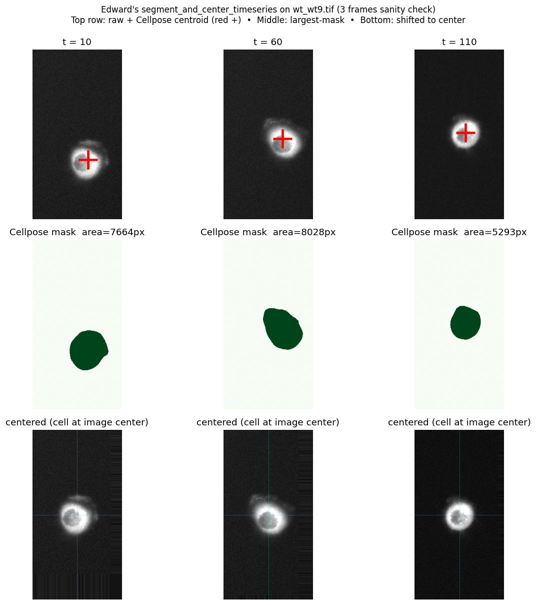
Top row: raw frame with the Cellpose centroid marked (red +). Middle row: the largest mask Cellpose found. Bottom row: the same frame shifted so the cell sits at image centre.
- Cellpose finds the cell on every frame with
model_type='cyto'and default diameter (zero-shot, no fine-tuning). - Mask area drops 8028 → 5293 px (t=60 → t=110), a 34% reduction. Consistent with active ring contraction.
- Centroid drifts ~70 px across the time-lapse, confirming that drift correction is necessary before computing per-cell metrics.
- CPU speed: 12.6 s/frame. Full 30-file dataset on CPU would take ~2.6 hours. Moved to GPU partition (
falcon/gecko) via sbatch (~5 min on GPU).
The full pipeline (raw .tif → migration metrics + lam/cyto ratio)
The full pipeline turns raw .tif time-lapses into per-cell biology metrics in five stages. Each stage writes its outputs to disk, so any downstream stage can be re-run independently.
raw .tif (T, H, W) uint16
    │
    │  (1) is_low_batch?  per-stack p99 < 1000
    │       yes → per-frame 1-99 percentile stretch
    │       no  → pass raw image through
    ▼
img_for_seg
    │
    │  (2) Cellpose (fine-tuned cyto3) .eval(diameter=None, channels=[0,0])
    │       largest connected mask → binary mask
    │       fallback if no mask → reuse last known centroid
    ▼
per-frame mask + centroid (cy, cx)
    │
    │  (3) shift image by (H/2 - cy, W/2 - cx) so the cell sits at frame centre
    ▼
centered .tif + mask .tif + centering_manifest.json (centers, n_empty, ...)
    │                                            │
    │  (4) Migration analysis                    │  (5) Lamellipodia analysis
    │      from manifest centers + masks         │      per-frame, inside the mask:
    │      mask-stability filter (area, IoU)     │      threshold = median(pixel)
    │      compute speed, path, net, persistence │      lam = mean(pixels ≥ threshold)
    │                                            │      cyto = mean(pixels < threshold)
    │                                            │      ratio = lam / cyto
    ▼                                            ▼
migration_metrics.csv                    per_cell_summary.csv (lam/cyto)
step 05Migration analysis
From per-frame centroids → speed, persistence, path length, net displacement
- Read the per-frame centroid trail from
centering_manifest.json(one (row, col) pixel coordinate per frame). - Step distance for each frame pair: the straight-line distance in pixels from one frame's centroid to the next.
- Convert to physical units: multiply by pixel size
0.318 µm/px; divide by frame interval60 sto get speed in µm/min. - Total path length: sum of all valid step distances (cumulative travel through every wiggle).
- Net displacement: straight-line distance from the very first valid centroid to the very last (start to end, ignoring the path in between).
- Persistence index = net displacement / total path length, capped at 1. 1 = perfectly straight trajectory; 0 = pure random walk. The cap defends against the rare case where one noisy step inflates net beyond path.
- Mean / median speed = average / median of all valid per-frame step speeds.
Mask-stability filter (why wt1/33 needed it)
wt1/33 initially reported a suspicious 5.55 µm/min. On inspection, Cellpose was fragmenting the mask in some frames — the centroid would jump from a 10,000-pixel mask to a 200-pixel fragment and back, producing fake 30 µm/min "displacements". A per-pair stability filter was added:
- A frame is valid only if its mask area is at least 30% of the per-cell median.
- A pair is valid only if both frames are valid and consecutive masks overlap with IoU ≥ 0.3.
After filtering, the worst single-frame jumps drop out and wt1/33 reports 1.88 µm/min — back in line with the rest of WT.
Per-condition summary (fine-tuned masks + mask-stability filter)
| Condition | Mean speed (µm/min) | Persistence | Total path | Net displacement |
|---|---|---|---|---|
| WT | 1.03 ± 0.33 | 0.31 ± 0.16 | 178 ± 103 µm | 43 ± 21 µm |
| KO | 1.06 ± 0.29 | 0.38 ± 0.17 | 204 ± 100 µm | 71 ± 48 µm |
| KI | 0.68 ± 0.08 | 0.31 ± 0.14 | 159 ± 58 µm | 50 ± 27 µm |
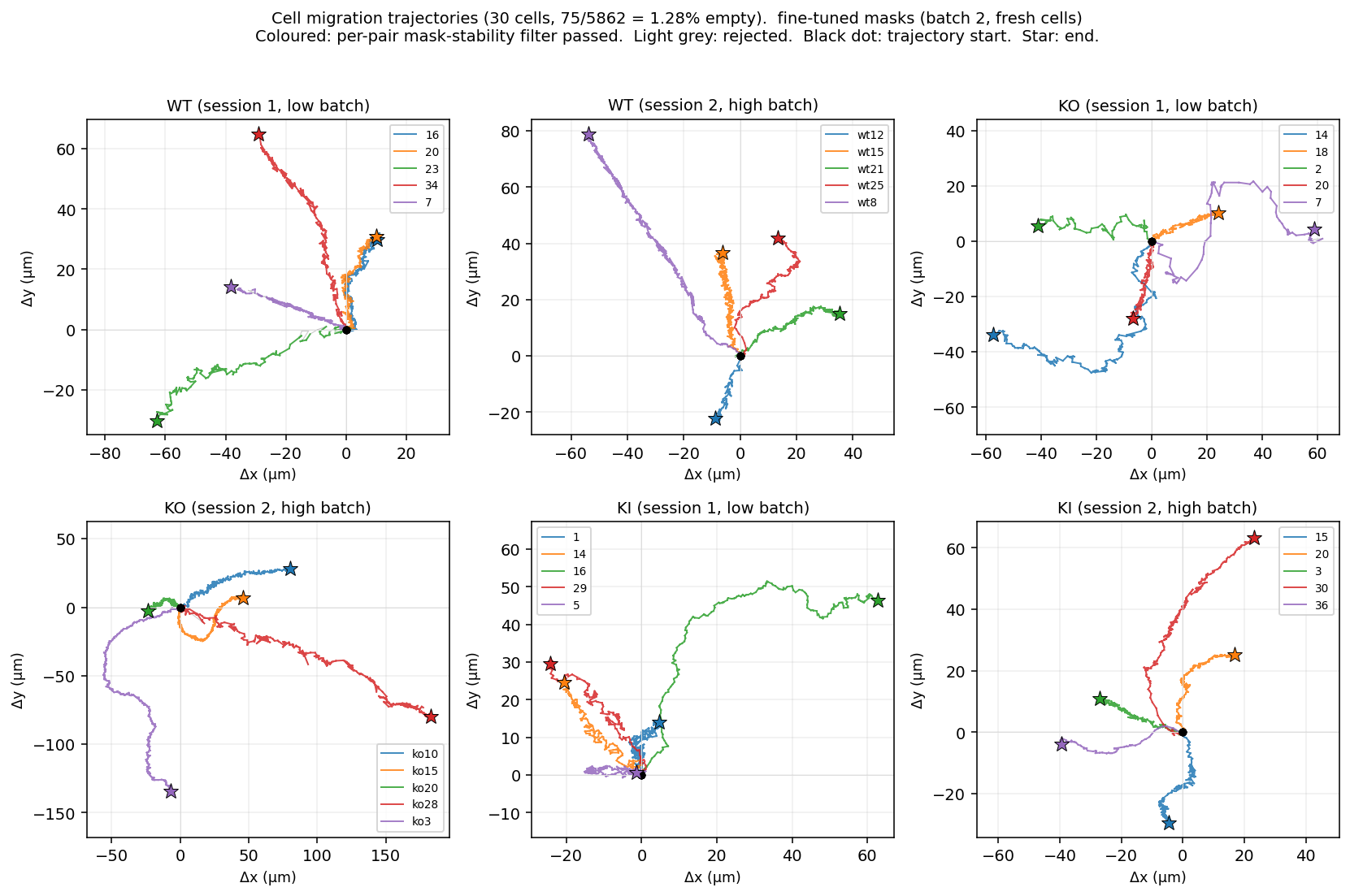
Trajectory visualisation
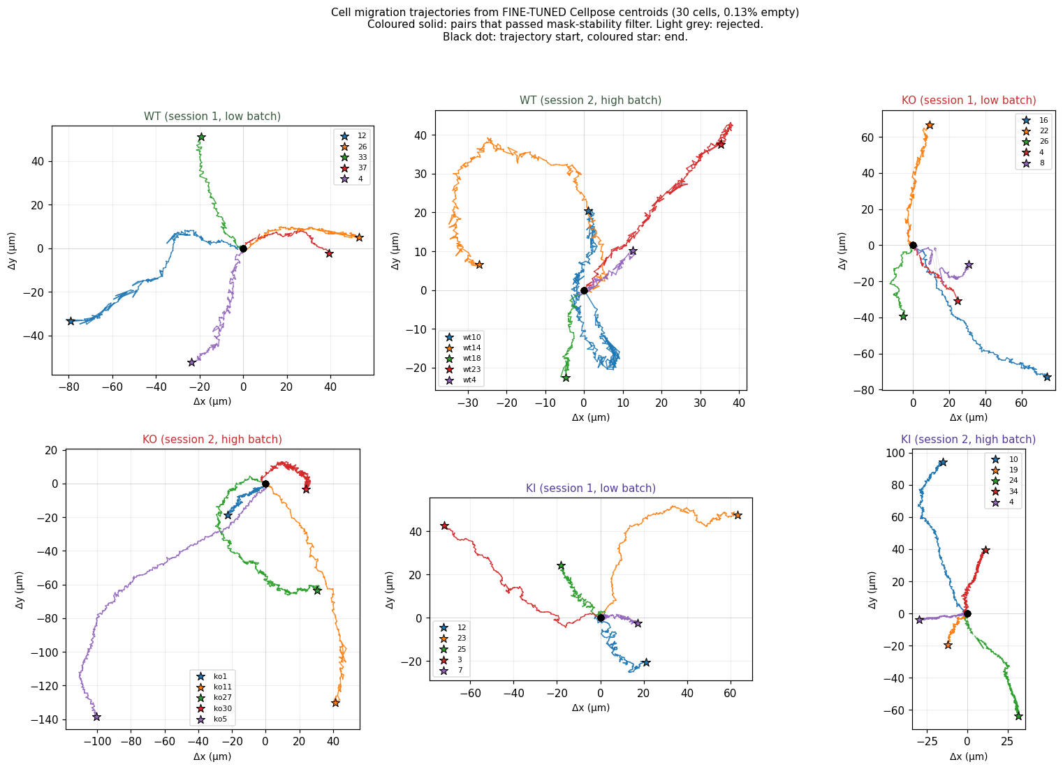
Each subplot is one folder, each coloured line is one cell, drawn from its starting position. Black dot = trajectory start, coloured star = end. Equal aspect ratio across panels; axes in microns. KI cells (bottom row) visibly travel shorter distances than WT (top) or KO (middle).
- N=10 per condition (5 cells × 2 imaging sessions). Variability is large; statistical tests pending.
ko1/4has 95% empty masks so it has zero valid pairs after filtering and contributes nothing to the KO summary.- Imaging session is a confound; the next pass should fit a mixed-effects model with batch as a random effect.
- The mask-stability filter is conservative (IoU ≥ 0.3). A handful of cells (
wt1/33,wt1/12,wt2/wt10,ko1/8) have many frames excluded; their reported metrics rely on the surviving valid pairs. - No photobleaching correction yet.
step 06Lamellipodia analysis
Split the cell mask at its own median pixel intensity → brighter half = lamellipodia signal
- For every frame, look only at the pixels inside the cell mask (ignore background and pixels outside the mask).
- Take the median intensity of those mask-interior pixels — this is the per-frame threshold τ.
- Split the mask in two:
- Brighter half (pixels ≥ τ): treated as the lamellipodium signal — Arp2/3 concentrated at the leading edge.
- Dimmer half (pixels < τ): treated as the cytoplasmic pool.
- Per-frame ratio = mean intensity of brighter half / mean intensity of dimmer half. Higher ratio = Arp2/3 more strongly concentrated at the cell front.
- Per-cell ratio = average of all per-frame ratios across non-empty frames.
The split is symmetric (brighter half vs dimmer half), so the ratio is unitless and partially robust to photobleaching: both halves decay together, and the ratio of their means changes much more slowly than either mean alone.
Choosing the split direction (parameter sweep)
Before committing to the dataset-wide run, we ran a parameter sweep on wt2/wt4.tif covering both directions and three percentile values, plus Multi-Otsu and a distance-transform variant.
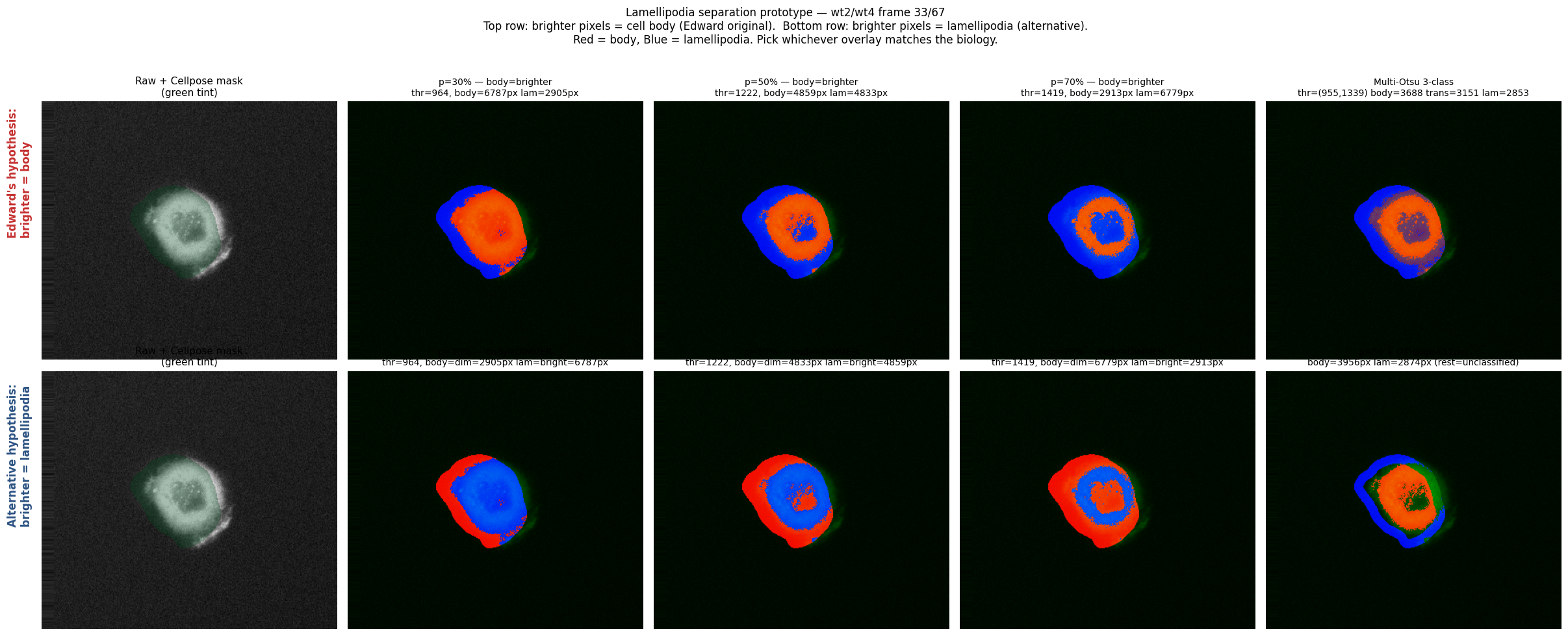
Red = cell body, Blue = lamellipodia in every overlay. Top row: original convention (brighter = body). Bottom row: swapped (brighter = lamellipodia). Top right: Multi-Otsu 3-class. Bottom right: percentile + distance-transform constraint (lamellipodia only within ~12 px of the cell boundary).
Direction confirmed: brighter pixels = lamellipodia (Arp2/3 concentrates at the leading edge). The bottom row of the prototype is the correct convention. Median split (percentile 50) was chosen for the dataset run because it balances signal-to-noise without introducing per-frame thresholding instability.
Full-dataset analysis on 30 cells (fine-tuned masks, percentile 50 split)
Per-cell mean intensity ratio of the brighter half (lamellipodia) to the dimmer half (cytoplasm). Higher ratio means Arp2/3 is more strongly concentrated at the cell edge.
| Condition | Lam / cyto intensity ratio | Cohen's d vs WT |
|---|---|---|
| WT | 1.53 ± 0.29 | baseline |
| KO | 1.47 ± 0.45 | −0.16 (similar) |
| KI | 1.83 ± 0.33 | +0.96 (large) |
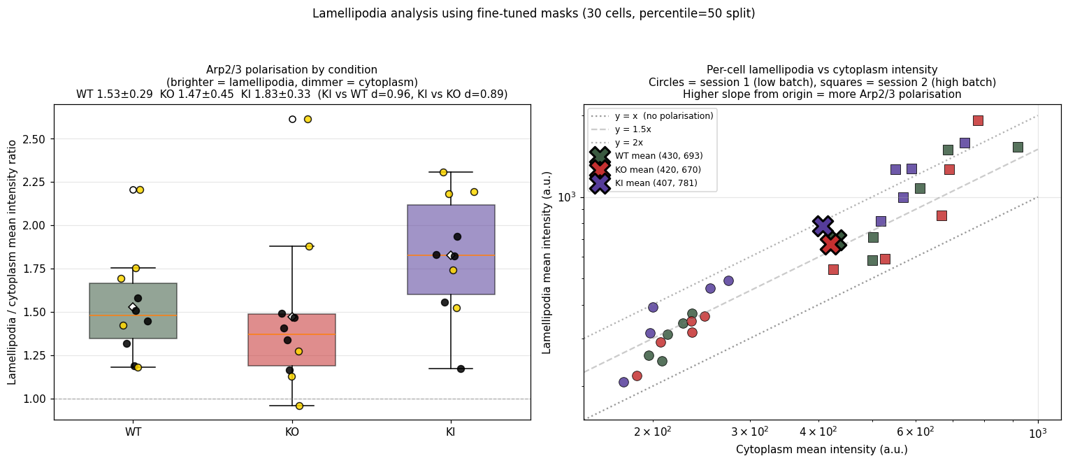
Left: per-cell ratio by condition. Right: per-cell lam_I vs cyto_I scatter (log axes); higher slope from origin = more polarisation. Circles = session 1 (low batch), squares = session 2 (high batch).
step 07Finding 1 · KI cells migrate ~35% slower
0.68 µm/min vs ~1.0 in WT/KO · Cohen's d > 1.4 (very large) · KI std collapses 7.5× after fine-tuning
Headline numbers
| Condition | Mean speed (µm/min) | Persistence | Cohen's d (vs WT) |
|---|---|---|---|
| WT | 1.03 ± 0.33 | 0.31 ± 0.16 | baseline |
| KO | 1.06 ± 0.29 | 0.38 ± 0.17 | +0.10 (similar) |
| KI | 0.68 ± 0.08 | 0.31 ± 0.14 | −1.40 (very large) |
What this shows
- Normal (WT) cells and gene-deleted (KO) cells migrate at similar speeds (~1.0 µm/min, no statistically meaningful difference). Both are reasonably mobile.
- KO cells walk straighter than normal cells (persistence 0.38 vs 0.31). With impaired adhesion their trajectories are less wobbly — possibly because they cannot make the complex curving motions WT cells do.
- KI cells are dramatically slower (0.68 vs 1.0 µm/min). They are also remarkably consistent in being slow (very small variability across cells, std 0.08). Combined with the lamellipodia analysis (next step), this is the cleanest single biological signal in the dataset.
The 7.5× std collapse — why fine-tuning matters here
Before self-training, KI's per-cell speed std was 0.60 µm/min (mostly mask-fragmentation noise). After fine-tuning, it dropped to 0.08 µm/min — a 7.5× reduction. The mean barely moved, but the spread shrank dramatically. That is the signature of removing measurement noise while preserving signal. The slow-KI phenotype is so consistent across cells that variability collapses once segmentation noise is removed.
Per-condition migration metrics before (orange, off-the-shelf cyto3) and after self-training (purple). Error bars are standard deviations across cells. KI's std collapses 7.5×, revealing the consistent slow-migration phenotype.
KI cells (bottom row) visibly travel shorter distances than WT (top) or KO (middle). All 6 folders, equal aspect ratio, axes in microns.
step 08Finding 2 · KI cells over-polarise Arp2/3
lam/cyto ratio 1.83 vs ≈1.5 in WT/KO · Cohen's d ~0.9 (large)
Headline numbers
| Condition | Lam / cyto intensity ratio | Cohen's d (vs WT) |
|---|---|---|
| WT | 1.53 ± 0.29 | baseline |
| KO | 1.47 ± 0.45 | −0.16 (similar) |
| KI | 1.83 ± 0.33 | +0.96 (large) |
What this shows
- WT and KO are statistically indistinguishable in lamellipodia polarisation (ratio ~1.5, Cohen's d effectively zero).
- KI cells over-polarise — their Arp2/3 is more strongly concentrated at the leading edge than in normal cells. The lamellipodia push-machinery is over-activated, not under-activated.
- This is the surprising part. KI cells are worse migrators (step 07) but appear more aggressive at the protrusion stage. The contradiction is the whole story — see step 09.
Left: per-cell ratio by condition. Right: per-cell lam_I vs cyto_I scatter (log axes); higher slope from origin = more polarisation. Circles = session 1 (low batch), squares = session 2 (high batch). KI sits visibly above the WT/KO cloud on both panels.
Robustness
- The ratio is unitless (mean intensity over mean intensity), so absolute brightness differences between imaging sessions don't enter directly.
- The ratio is partially robust to photobleaching: both halves of the mask decay together, so the ratio of their means changes much more slowly than either mean alone. Absolute intensity numbers should still be read with caution; ratios less so.
- Both batches are visible in the right scatter (circles vs squares), and KI sits above WT/KO regardless of session — the finding holds across imaging conditions.
step 09Combined story · KI = broken protrusion–adhesion coordination
Dominant-negative phenotype · over-polarised Arp2/3 + slowest migration · more damaging than full deletion
Two complementary findings about KI
- KI cells over-polarise Arp2/3 to the leading edge (lam/cyto ratio 1.83 vs ≈1.5 in WT/KO, Cohen's d ~0.9).
- KI cells migrate dramatically slower than WT/KO (0.68 vs 1.0 µm/min, Cohen's d > 1.4).
Why this combination is meaningful
Together this is exactly what "broken protrusion–adhesion coordination" predicts: the protrusion machinery activates more strongly than normal (more Arp2/3 at the edge) yet the cell cannot translate this into productive migration. Without functional adhesion-protrusion coordination, the lamellipodia keeps forming but cannot generate traction. Consistent with the KI point mutation producing a non-functional product that interferes with the migration machinery rather than simply being absent.
The 4-step migration model — where KI breaks down
Cell migration is canonically described in 4 steps:
- Protrusion — push the front edge forward (driven by Arp2/3-nucleated branched actin = lamellipodium).
- Adhesion — anchor the new front edge to the substrate.
- Traction — generate pulling force using the anchored front.
- Release — detach the rear and let the cell move forward.
The perturbed gene matters for both step 1 (protrusion) and step 2 (adhesion). So the three conditions break down differently:
| Condition | Step 1 protrusion | Step 2 adhesion | Net migration |
|---|---|---|---|
| WT | normal | normal | ~1.0 µm/min, polarisation 1.53 |
| KO | ~normal | impaired | ~1.0 µm/min (similar to WT), polarisation 1.47 trajectories straighter — fewer complex curves |
| KI | over-active | broken coordination | 0.68 µm/min (~35% slower), polarisation 1.83 protrusion machinery fires harder than normal yet productive migration drops |
Why KO is less damaging than KI
This is the counterintuitive part of the result. A complete deletion (KO) of the gene preserves migration speed almost perfectly. A point mutation (KI) does not. The most plausible interpretation:
- KO produces nothing at the protein-of-interest's slot. Migration still works because compensatory pathways or partner proteins compensate; the cell just walks slightly less wobbly (higher persistence 0.38 vs 0.31).
- KI produces a defective protein that occupies the slot but doesn't function correctly. It still binds the migration machinery and over-activates the protrusion stage, but cannot transduce that into adhesion + traction. This is the classic dominant-negative signature — a broken part is worse than a missing part because the broken part still interferes.
What we still don't know about the gene itself
We have not been told which gene specifically is perturbed in KO and KI. The function is described (protrusion + adhesion coordination) but the gene is not named. Knowing the gene would let us cross-check our finding against published phenotypes — for example, whether published KO/KI phenotypes match the slow-migration + over-polarised pattern we observe. Worth asking the biology lead before drawing further conclusions.
step 10Generalisation test · fresh 30 cells
Same fine-tuned model, no retraining, applied to 30 cells the model never saw · both findings reproduce
Setup
After the main analysis was complete, a second upload of 30 fresh cells arrived (same 6 categories: wt1, wt2, ko1, ko2, ki1, ki2, 5 cells each, 5,862 frames in total). These cells were never seen by the fine-tuned Cellpose model. Re-running the full pipeline on them is a strong test of whether the model and the biological findings hold up beyond the cells used during self-training.
- Same fine-tuned
cyto3model (no retraining, no parameter changes). - Same adaptive 1–99 percentile normalize (only applied to low-batch files, judged by per-stack p99 < 1000).
- Same migration filter: mask area ≥ 30% of per-cell median, IoU ≥ 0.3 between consecutive frames.
- Same lamellipodia split: percentile 50 inside the mask, brighter pixels treated as lamellipodia.
Segmentation quality on unseen cells
| Batch | Cells | Frames | Empty masks | Empty rate |
|---|---|---|---|---|
| Batch 1 (original 30) | 30 | 6,221 | 8 | 0.13% |
| Batch 2 (fresh 30) | 30 | 5,862 | 75 | 1.28% |
The empty-mask rate on fresh cells is ~10× higher relative (9.95×: 1.28% vs 0.13%) but still under 2% absolute. 25 of 30 fresh cells had zero empty masks. Five had non-zero rates, with one hard case ko1/7 at 28.3% (30/106 frames). Expected pattern: fine-tuning generalises broadly but does not solve every imaging artefact.
Findings reproduce on fresh data
| Metric | Batch 1 (original) | Batch 2 (fresh) | Reproduces? |
|---|---|---|---|
| Migration speed (µm/min) | |||
| WT | 1.03 ± 0.33 | 0.95 ± 0.24 | yes |
| KO | 1.06 ± 0.29 | 1.19 ± 0.43 | yes |
| KI | 0.68 ± 0.08 | 0.72 ± 0.10 | yes (KI slowest in both) |
| Lamellipodia / cytoplasm intensity ratio | |||
| WT | 1.53 ± 0.29 | 1.60 ± 0.37 | yes |
| KO | 1.47 ± 0.45 | 1.64 ± 0.56 | yes |
| KI | 1.83 ± 0.33 | 1.83 ± 0.27 | yes — KI means agree to within 0.003 (1.827 vs 1.830) |
| Cohen's d (effect size) | |||
| Migration KI vs WT | −1.40 | −1.22 | yes (very large in both) |
| Migration KI vs KO | −1.68 | −1.44 | yes (very large in both) |
| Lam ratio KI vs WT | +0.90 | +0.67 | yes (medium to large) |
| Lam ratio KI vs KO | +0.85 | +0.41 | yes (same direction, weaker) |
Per-cell migration trajectories on the fresh batch. 6 folders, 5 cells each. Coloured polylines: per-pair mask-stability filter passed. Light grey: rejected. Black dot: trajectory start, coloured star: end. KI cells (last two panels) cover noticeably shorter ground than WT and KO — the same pattern observed on batch 1.
What this means
The biological story (KI cells migrate slower while paradoxically over-polarising Arp2/3 to the leading edge) holds up on cells the model has never seen. The KI mean lam/cyto ratio is 1.827 in batch 1 and 1.830 in batch 2: the two means agree within 0.003 on independent groups of 10 cells. With samples this small this is not formal proof, but agreement on independent data is a strong signal that the result is not specific to the cells used during self-training.
- The KI dominant-negative finding is consistent across both batches, which makes a model-fitting artefact unlikely.
- The fine-tuned segmentation model handles unseen cells in this dataset family well enough that retraining is probably unnecessary for routine analysis.
- This is a generalisation test, not a formal cross-validation. The original 30 cells were used to filter self-training data, so they are not strictly held out — see step 11 for an independent cross-validation against a biologist-trained model.
- Statistical significance was not formally tested. A mixed-effects ANOVA with batch as a random effect would be the next step.
- Five batch-2 cells had non-zero empty rates.
ko1/7in particular is a hard case (28.3% empty, 30 of 106 frames) and worth a manual look.
step 11Cross-validation under a biologist-trained model
Day 3 morning · 14 cells with Quimp active-contour reference masks · independent Cellpose model · KI finding holds
Result: two completely independent segmentation philosophies (deep-learning self-trained on filtered v3 outputs vs Cellpose trained on Quimp active-contour biologist masks) converge on essentially the same KI lam/cyto ratio (1.83–1.88) and the same Cohen's d (~+0.9). The dominant-negative interpretation is not an artefact of the self-training pseudo-ground-truth.
Headline figure · all 16 effect-size bars point the same way
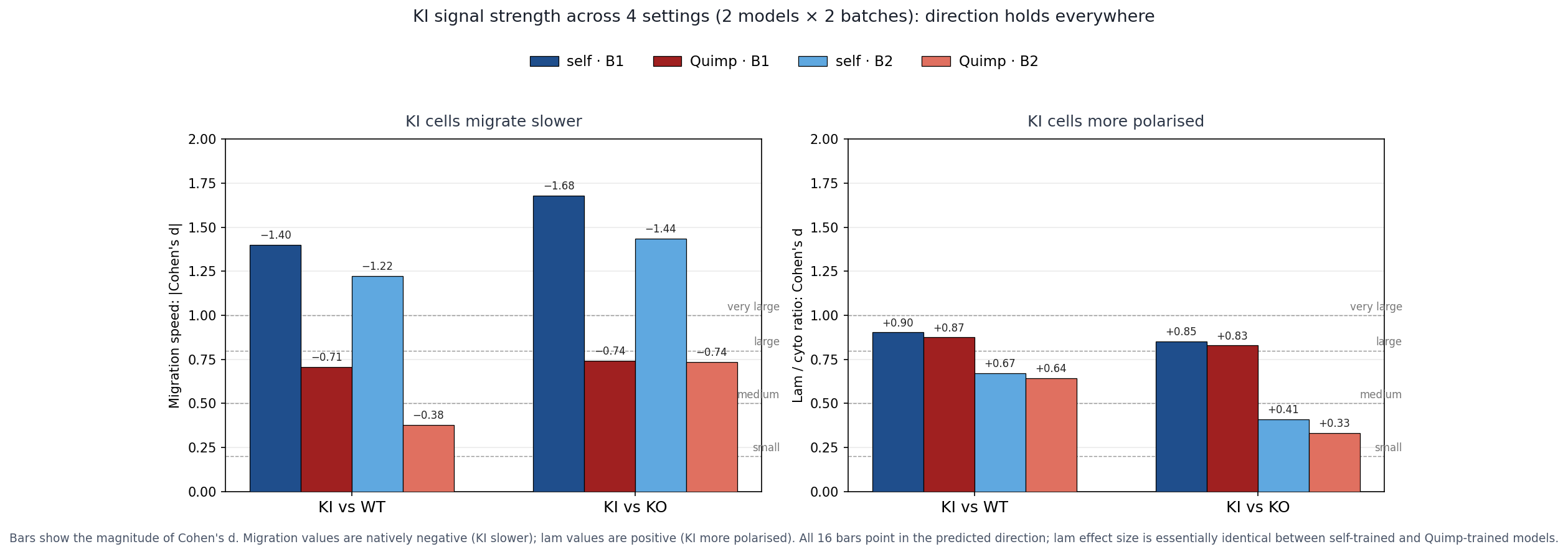
Two panels (migration, lamellipodia) × four model×batch combinations. All 16 bars align with the predicted direction. The lamellipodia panel is nearly identical between the two models; migration effect-sizes shrink slightly under Quimp because its larger boundary inflates within-condition variance, but the direction is preserved.
Setup
- 14 cells, ~2,500 frame-mask pairs after stride-5 sampling, un-shifted from Quimp's centered frame back to raw frame.
- Same hyperparameters as self-training:
cyto3base, 100 epochs, SGD lr=0.05. - Train loss 0.335 → 0.014 in 9 minutes on RTX A5000.
- Inference on all 60 cells (batch 1 + batch 2): ~17 minutes.
Empty-mask rate (segmentation quality)
| Model | Batch 1 | Batch 2 |
|---|---|---|
| Self-trained | 0.13% | 1.28% |
| Quimp-trained | 2.12% | 1.40% |
Quimp model is slightly less aggressive on Batch 1 (only 14 of 30 cells were in its training set; the rest are unseen). Both stay under 2.5% — production-grade quality.
Boundary-philosophy comparison · the two models on the same cells
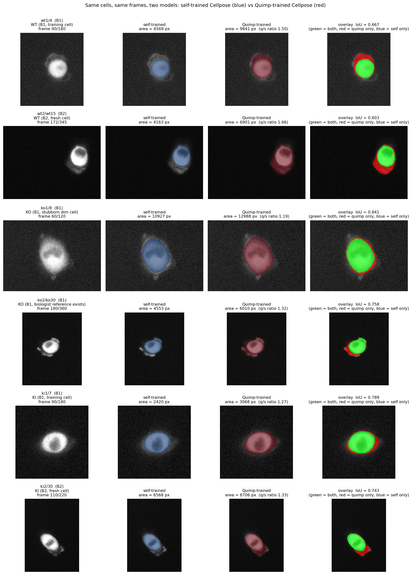
Six representative cells. Self-trained model produces tighter cell-body boundaries. Quimp-trained version captures more of the peripheral halo (mean area ratio ~1.17×). Same biology, different definitions of where the cell ends — this is what shifts the migration Cohen's d down without changing direction.
Lamellipodia / cytoplasm intensity ratio (the headline cross-check)
| Condition | self_b1 | quimp_b1 | self_b2 | quimp_b2 |
|---|---|---|---|---|
| WT | 1.53 ± 0.29 | 1.56 ± 0.34 | 1.60 ± 0.37 | 1.63 ± 0.40 |
| KO | 1.47 ± 0.45 | 1.50 ± 0.50 | 1.64 ± 0.56 | 1.70 ± 0.59 |
| KI | 1.83 ± 0.33 | 1.88 ± 0.35 | 1.83 ± 0.27 | 1.86 ± 0.29 |
KI lam/cyto ratio reproduces with essentially identical magnitude across both models on both batches (1.83–1.88). Cohen's d for KI vs WT: +0.90 (self_b1) versus +0.87 (quimp_b1); +0.67 (self_b2) versus +0.64 (quimp_b2). The two segmentation philosophies converge on the same number.
Migration speed (µm/min)
| Condition | self_b1 | quimp_b1 | self_b2 | quimp_b2 |
|---|---|---|---|---|
| WT | 1.03 ± 0.33 | 1.04 ± 0.45 | 0.95 ± 0.24 | 1.03 ± 0.34 |
| KO | 1.06 ± 0.29 | 1.36 ± 1.01 | 1.19 ± 0.43 | 1.20 ± 0.48 |
| KI | 0.68 ± 0.08 | 0.79 ± 0.14 | 0.72 ± 0.10 | 0.91 ± 0.21 |
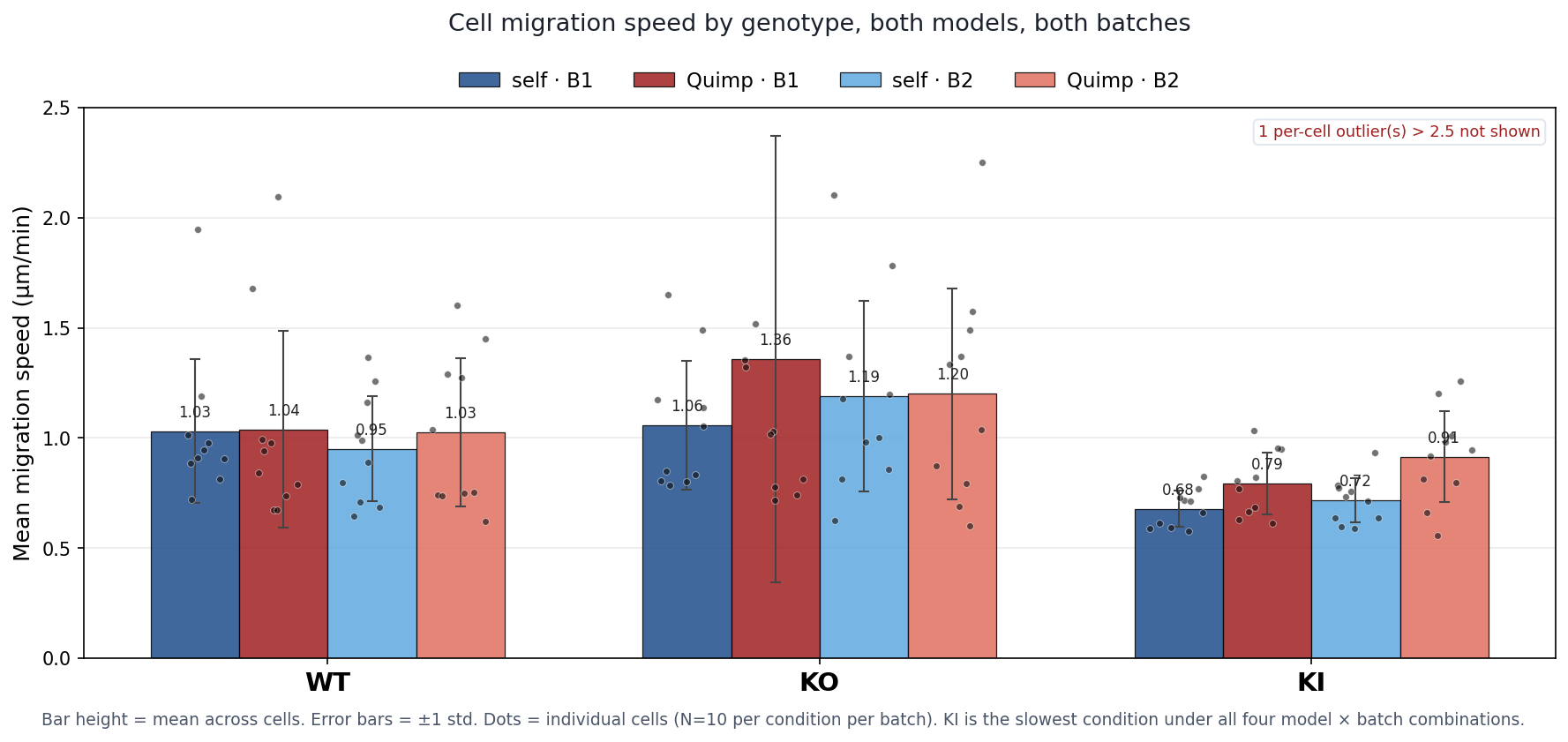
Mean migration speed (bars) with per-cell dots overlaid. Three conditions × two models × two batches. y-axis capped at 2.5 µm/min (one outlier excluded for readability). KI is the slowest condition under all four model × batch combinations.
Cohen's d for migration KI vs WT shifts from "very large" (−1.40 self_b1) to "medium-large" (−0.71 quimp_b1) because Quimp's larger boundary makes the centroid more sensitive to halo shape changes, which inflates within-condition variance. The direction of the finding is preserved.
Trajectories under the Quimp-trained model (both batches)
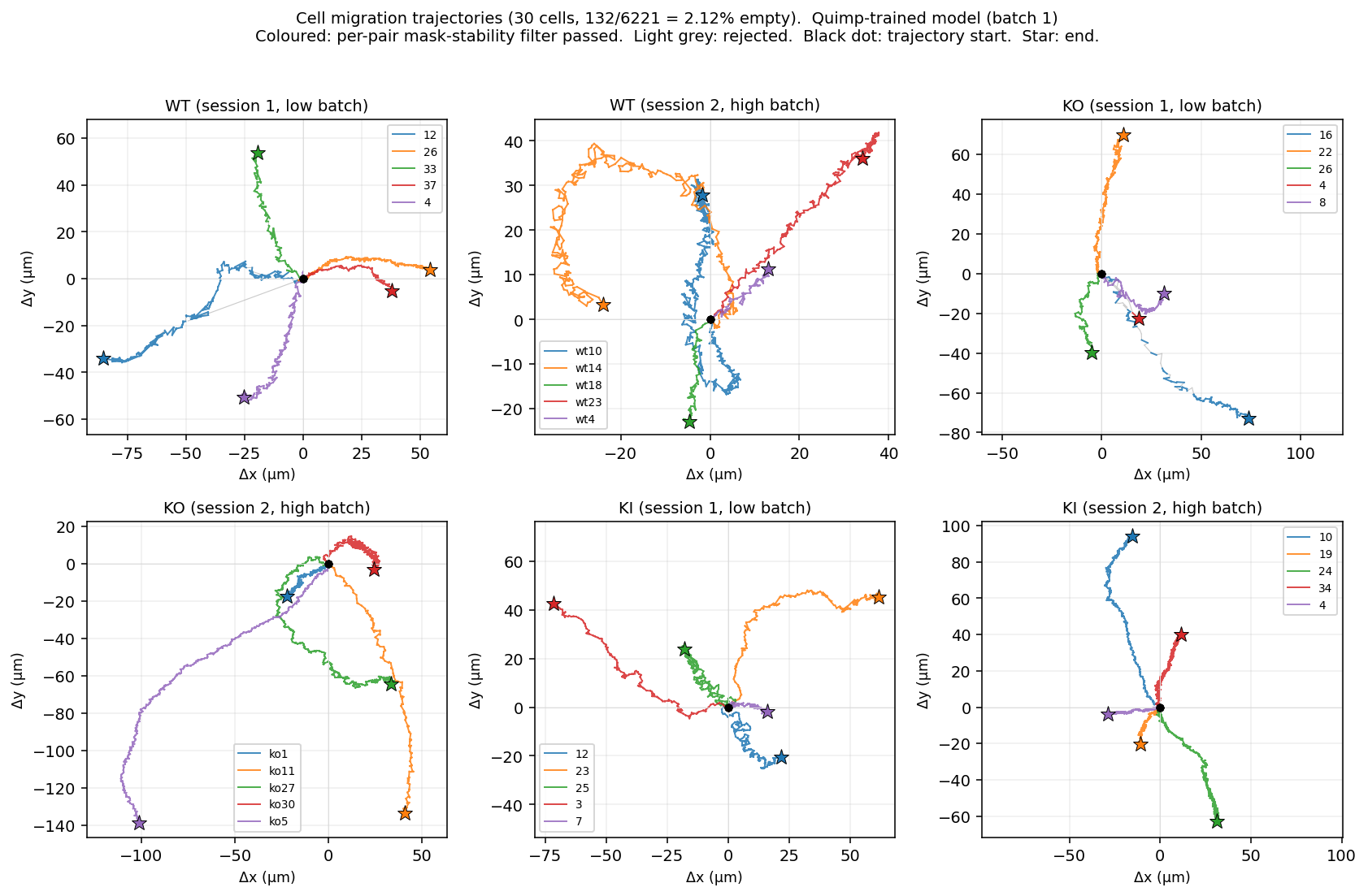
Batch 1 (original 30 cells)
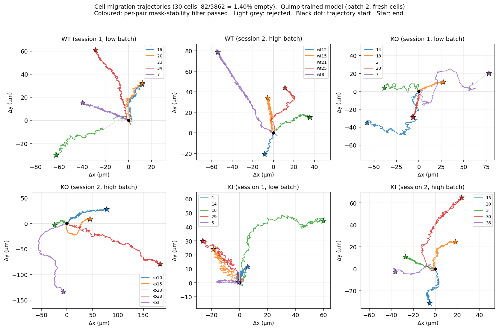
Batch 2 (fresh 30 cells)
KI cells (last two panels in each batch) cover noticeably less ground than WT and KO across both batches under the Quimp model — same pattern observed under the self-trained model in steps 05 and 10.
Conclusion
What we accomplished (full hackathon)
- Pipeline: off-the-shelf Cellpose at 9.7% empty masks → self-trained pipeline at 0.13% empty masks (a 75-fold improvement).
- Migration finding: KI cells migrate roughly 35% slower than WT or KO (Cohen's d > 1.4 in the original analysis, holds across all 4 model × batch combinations).
- Lamellipodia finding: KI cells over-polarise Arp2/3 (lam/cyto ratio 1.83 vs ~1.5, Cohen's d ~0.9; agreement to within 0.003 between batches).
- Combined biological story: the KI mutation produces hyperactive forward-push machinery that the cell cannot translate into actual migration — dominant-negative phenotype, more damaging than full deletion.
- Reusable tools: generic two-mask comparison utility (IoU / Dice / HD95), ready for any future ground-truth annotation.
- Generalisation (step 10): same fine-tuned model on 30 fresh cells — empty rate < 2%, both findings reproduce, KI mean lam/cyto ratio agrees to 0.003 between batches.
- Cross-validation (this step): independent Cellpose model trained on biologist Quimp masks reaches the same KI ratio and Cohen's d. The finding is not a self-training artefact.
- Reproducible: all code, data manifests, processed outputs, both trained models (self + Quimp, 26 MB each), and figures in the public GitHub repo.
What we still don't know
Worth asking the biology lead to make the findings sharper:
- What gene specifically is perturbed in KO and KI? The function is described (protrusion + adhesion coordination) but the gene is not named. Knowing the gene would let us cross-check our finding against published phenotypes.
- Are
ko1/4andko1/8technical or biological? Both have very dim fluorescence.ko1/4stopped after 60 frames (possibly aborted);ko1/8stays consistently dim. Either source-data limitation or a genuine phenotype. - How many "layers" inside the cell do you want quantified? We currently split each cell into 2 (lamellipodia at the edge vs cytoplasm). Could refine to 3 (body / transition zone / lamellipodia) if needed.
- Why does
ko1/7still fail on the fresh batch? Model handled 25 of 30 fresh cells with zero empty masks but flagged this one with 28.3% empty. Worth a manual look.
Future work (ran out of time for)
- Formal statistical tests — mixed-effects model with imaging session as a random effect, to give p-values rather than effect sizes alone.
- Photobleaching correction — GFP fluorescence decays with cumulative laser exposure. Absolute intensity numbers should be read with caution; ratios (lam/cyto) are partially robust because both populations decay together.
- More biologist Quimp annotations — currently 14 cells; expanding to 60 would let the Quimp-trained model fully replace the self-trained one and provide a proper ground-truth IoU benchmark.
- Interactive viewer — a napari-based dashboard for the biology team to browse cells and inspect segmentation interactively.